Radius of convergence
In mathematics, the radius of convergence of a power series is a quantity, either a non-negative real number or ∞, that represents a domain (within the radius) in which the series will converge. Within the radius of convergence, a power series converges absolutely and uniformly on compacta as well. If the series converges, it is the Taylor series of the analytic function to which it converges inside its radius of convergence.
Contents |
Definition
For a power series ƒ defined as:
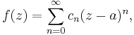
where
- a is a complex constant, the center of the disk of convergence,
- cn is the nth complex coefficient, and
- z is a complex variable.
The radius of convergence r is a nonnegative real number or ∞ such that the series converges if

and diverges if
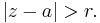
In other words, the series converges if z is close enough to the center and diverges if it is too far away. The radius of convergence specifies how close is close enough. On the boundary, that is, where |z − a| = r, the behavior of the power series may be complicated, and the series may converge for some values of z and diverge for others. The radius of convergence is infinite if the series converges for all complex numbers z.
Finding the radius of convergence
Two cases arise. The first case is theoretical: when you know all the coefficients  then you take certain limits and find the precise radius of convergence. The second case is practical: when you construct a power series solution of a difficult problems you typically will only know a finite number of terms in a power series, anywhere from a couple of terms to a hundred terms. In this second case, extrapolating a plot estimates the radius of convergence.
Theoretical radius
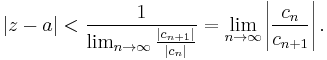
The radius of convergence can be found by applying the root test to the terms of the series. The root test uses the number
![C = \limsup_{n\rightarrow\infty}\sqrt[n]{|c_n(z-a)^n|} = \limsup_{n\rightarrow\infty}\sqrt[n]{|c_n|}|z-a|](/2012-wikipedia_en_all_nopic_01_2012/I/8556c016de54f3f486d3901fc7058986.png)
"lim sup" denotes the limit superior. The root test states that the series converges if C < 1 and diverges if C > 1. It follows that the power series converges if the distance from z to the center a is less than
![r = \frac{1}{\limsup_{n\rightarrow\infty}\sqrt[n]{|c_n|}}](/2012-wikipedia_en_all_nopic_01_2012/I/e59ac417d852ff5c18fe14f655501bab.png)
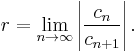
and diverges if the distance exceeds that number; this statement is the Cauchy–Hadamard theorem. Note that r = 1/0 is interpreted as an infinite radius, meaning that ƒ is an entire function.
The limit involved in the ratio test is usually easier to compute, and when that limit exists, it shows that the radius of convergence
This is shown as follows. The ratio test says the series converges if
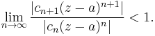
That is equivalent to
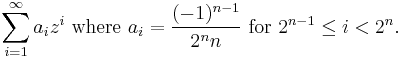
Practical estimation of radius
Suppose you only know a finite number of coefficients , say ten to a hundred. Typically, as  increases, these coefficients settle into a regular behavior determined by the nearest radius-limiting singularity.
When the behavior of the coefficients is one of constant sign or alternating sign, Domb and Sykes[1] proposed plotting  against
  , fitting a straight line extrapolation, and taking the intercept of this line as an estimate the reciprocal
  of the radius of convergence. Negative
  means the convergence-limiting singularity is on the negative axis. Naturally, this is called a Domb-Sykes plot.
When the coefficients settle into having a periodic pattern of signs then use a test proposed by Mercer and Roberts.[2] Compute  from
from  and plot versus . Extrapolate to
  to again estimate the reciprocal of the radius of convergence.
You may also estimate two subsidiary quantities. Estimate the exponent  of the convergence limiting singularity because the slope of the straight line extrapolation is
  . Estimate the angle
  , from the real axis, of the convergence limiting singularities by plotting
  versus
  . Then extrapolating to
  estimates
  .
.
Radius of convergence in complex analysis
A power series with a positive radius of convergence can be made into a holomorphic function by taking its argument to be a complex variable. The radius of convergence can be characterized by the following theorem:
- The radius of convergence of a power series f centered on a point a is equal to the distance from a to the nearest point where f cannot be defined in a way that makes it holomorphic.
The set of all points whose distance to a is strictly less than the radius of convergence is called the disk of convergence.
The nearest point means the nearest point in the complex plane, not necessarily on the real line, even if the center and all coefficients are real. For example, the function
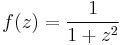
has no singularities on the real line, since  has no real roots. Its Taylor series about 0 is given by
The root test shows that its radius of convergence is 1. In accordance with this, the function ƒ(z) has singularities at ±i, which are at a distance 1 from 0.
For a proof of this theorem, see analyticity of holomorphic functions.
A simple example
The arctangent function of trigonometry can be expanded in a power series familiar to calculus students:
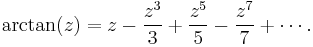
It is easy to apply the root test in this case to find that the radius of convergence is 1.
A more complicated example
Consider this power series:
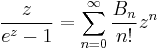
where the rational numbers Bn are the Bernoulli numbers. It may be cumbersome to try to apply the ratio test to find the radius of convergence of this series. But the theorem of complex analysis stated above quickly solves the problem. At z = 0, there is in effect no singularity since the singularity is removable. The only non-removable singularities are therefore located at the other points where the denominator is zero. We solve

by recalling that if z = x + iy and e iy = cos(y) + i sin(y) then

and then take x and y to be real. Since y is real, the absolute value of cos(y) + i sin(y) is necessarily 1. Therefore, the absolute value of e z can be 1 only if e x is 1; since x is real, that happens only if x = 0. Therefore z is pure imaginary and cos(y) + i sin(y) = 1. Since y is real, that happens only if cos(y) = 1 and sin(y) = 0, so that y is an integral multiple of 2π. Consequently the singular points of this function occur at
- z = a nonzero integer multiple of 2πi.
The singularities nearest 0, which is the center of the power series expansion, are at ±2πi. The distance from the center to either of those points is 2π, so the radius of convergence is 2π.
Convergence on the boundary
If the power series is expanded around the point a and the radius of convergence is r, then the set of all points z such that |z − a| = r is a circle called the boundary of the disk of convergence. A power series may diverge at every point on the boundary, or diverge on some points and converge at other points, or converge at all the points on the boundary. Furthermore, even if the series converges on the boundary, it does not necessarily converge absolutely.
Example 1: The power series for the function ƒ(z) = (1 − z)−1, expanded around z = 0, has radius of convergence 1 and diverges at every point on the boundary.
Example 2: The power series for g(z) = ln(1 − z) has radius of convergence r = 1 expanded around z = 0, and diverges for z = 1 but converges for all other points on the boundary. ƒ(z) in Example 1 is the derivative of the negative of g(z).
Example 3: The power series

has radius of convergence 1 and converges everywhere on the boundary. If h(z) is the function represented by this series, then the derivative of h(z) is g(z) divided by z in Example 2. It turns out that h(z) is the dilogarithm function.
Example 4: The power series
has radius of convergence 1 and converges uniformly on the boundary {|z| = 1}, but does not converge absolutely on the boundary.[3]
Comments on rate of convergence
If we expand the function
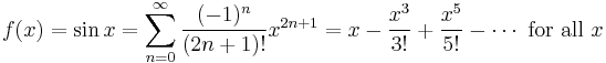
around the point x = 0, we find out that the radius of convergence of this series is  meaning that this series converges for all complex numbers. However, in applications, one is often interested in the precision of a numerical answer. Both the number of terms and the value at which the series is to be evaluated affect the accuracy of the answer. For example, if we want to calculate ƒ(0.1) = sin(0.1) accurate up to five decimal places, we only need the first two terms of the series. However, if we want the same precision for x = 1, we must evaluate and sum the first five terms of the series. For ƒ(10), one requires the first 18 terms of the series, and for ƒ(100), we need to evaluate the first 141 terms.
So the fastest convergence of a power series expansion is at the center, and as one moves away from the center of convergence, the rate of convergence slows down until you reach the boundary (if it exists) and cross over, in which case the series will diverge.
A graphical example
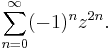
Consider the function 1/(z2 + 1).
This function has poles at z = ±i.
As seen in the first example, the radius of convergence of this function's series in powers of (z − 0) is 1, as the distance from 0 to each of those poles is 1.
Then the Taylor series of this function around z = 0 will only converge if |z| < 1, as depicted on the example on the right.
Abscissa of convergence of a Dirichlet series
An analogous concept is the abscissa of convergence of a Dirichlet series

Such a series converges if the real part of s is greater than a particular number depending on the coefficients an: the abscissa of convergence.
Notes
- ^ C. Domb and M. F. Sykes, On the susceptibility of a ferromagnet above the Curie point, Proc. Roy. Soc. Lond. A 240:214-228, 1957.
- ^ G. N. Mercer and A. J. Roberts, A centre manifold description of contaminant dispersion in channels with varying flow properties, SIAM J.~Appl. Math. 50:1547-1565, 1990.
- ^ Sierpiński, Wacław (1918), "O szeregu potęgowym który jest zbieżny na całem swem kole zbieżności jednostajnie ale nie bezwzględnie", Prace matematyka-fizyka 29: 263–266
References
- Brown, James; Churchill, Ruel (1989), Complex variables and applications, New York: McGraw-Hill, ISBN 978-0-07-010905-6
- Stein, Elias; Shakarchi, Rami (2003), Complex Analysis, Princeton, New Jersey: Princeton University Press, ISBN 0-691-11385-8